Due to the vast amount of operational parameters at play in tool manufacturing, cost and price calculation for custom tools and small lot sizes currently poses a major challenge for the industry. Only having built previous applications based on event sourcing unlocked the possibility for predicting relevant values based on previously collected historical data for price calculation.
This post describes how we enabled on-demand price calculation for customer-designed special milling cutters using machine learning (ML) based on data from traditional systems of record and event streams.
While the domain is very specific, the general approach for making sense of your event log and master data using machine learning can be applied just as well in different scenarios.
Setting the stage
At a medium-sized manufacturer for solid carbide milling cutters in Germany, several systems work together in the described scenario:
- An enterprise resource planning (ERP) system containing master data for offered products and orders.
- An event-sourced manual work logging solution for tracking activities on the shop floor.
- An interactive online configurator to design special tools. Customers can specify the desired basic geometry of the tool such as (amongst others) length, blade length, diameters, target materials, and the number of blades, which are presented in a corresponding technical drawing, and then customers can request a quote.
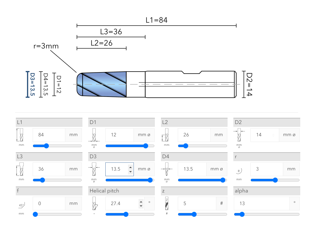
Figure 1: Online custom tool configurator
These tools have been developed largely independently of each other and have been used in production for several years.
Quotes for custom tools were handled manually: customers would configure a tool and request a quote. The configuration parameters were sent to the sales department which created an offer estimated mostly based on individual experience.
To further expand the custom tool business, the configurator should be extended to allow embedding and ordering directly in online shops. For that, a price for the configuration needs to be calculated dynamically on-demand, as opposed to specialized staff estimating it. Several components of the price calculation formula are obvious and easily defined. These include the price of raw materials and coating, the hourly rates of workers as well as surcharges accounting for scrap and set-up times. One important component, though, cannot be calculated in a simple fashion: the time a grinding machine takes to produce one piece for the given configuration.
Problem-solving approach
Currently, grinding times are not calculated but simulated. However the configuration parameters describe the basic geometry of the product, they are not sufficient to run such a simulation. Based on these parameters, a grinding program for a suitable machine needs to be devised which then, in turn, can be used to drive the simulation. Obviously, this approach is not feasible for an online shopping scenario. We need one capable of running without human interaction in a quick, fully automated fashion.
Expecting the geometry parameters to affect grinding times in a deterministic fashion is reasonable, according to our domain experts, even if we do not know yet which parameters have how large an influence.
After intense discussions on how to solve this programmatically, we learned that capturing all relevant operational parameters is such a huge undertaking that, as of today, none of our contacts in the industry has succeeded in doing so[1]. With a lot of effort and capturing and maintaining additional production master data, we could come up with reasonable estimates, but even these could be off significantly in edge cases. We wanted to do better than that. One of the domain experts, a bit frustrated for not making progress, voiced his sentiment:
“Why can’t we just pick a grinding time of a tool we’ve already produced similar to the configured one? And maybe tweak it a bit?”
This made us realize we actually had all the data required to do so at hand: the ERP system has the parameters for each offered product and the work logging system has the grinding times per workpiece for each order produced. When setting up the work logging system, we did know that grinding times were important, but hadn’t conceived the resulting data being used in this way. That’s one of the benefits of event-sourced systems: you end up with a treasure trove of data, the event log, that can be interpreted after the fact to answer questions that come up without even having considered the question at design time.
We were still left with the question of how to determine ‘similarity’ (which is a non-trivial problem in multidimensional data sets) and how to ‘tweak’ the result. Enter machine learning.
Formulated in machine learning terms, we’re facing a regression problem and can employ supervised learning: We want to predict grinding times for unknown geometries based on previously recorded grinding times for which we have the geometries at hand.
Armed with this approach and the data, the challenge seems significantly less daunting than it did as we set out.
Data aggregation
For the master data, we retrieved a simple CSV report from the ERP containing the article number of each product along with all customer-adjustable geometry parameters.
For known grinding times, the training data set, we created a projection in EventStoreDB that extracted the grinding times for each order along with the article number of the produced product. Luckily, the grinding times were recorded as part of the grinding.stopped event explicitly. But even if it hadn’t been, it would have been trivial to compute them based on ‘work started’ and ‘work stopped’ time per order. Since we hadn’t accounted for the data being used in this way, the projection also needed to include some additional clean-up to filter out events missing required data. We also needed to account for compensation events that happen if a worker corrects mistakes he made earlier. The slightly simplified source of the projection can be found in Listing 1.
Merging those two data sets based on the article number gives us a list of geometries along with the required grinding times. Since each product has been manufactured many times, these samples account for typical fluctuations in grinding times during production.
All of this was implemented in python within a Jupyter notebook[2] using the pandas library[3] which allows for easy data manipulation, even of large data sets.
Time to put on our data science hat and see what we can learn from that data set.
Data evaluation & cleansing
We won’t go into too much detail describing the milling cutter’s geometry parameters, but they shouldn’t be completely opaque either. Suffice to know that L1-L4 describe various lengths, D1-D3 diameters, alpha, r, f and sst angles, and z the number of blades. grinding_time_min is the feature we’re trying to predict: The grinding time in minutes.
When training ML models, sample size and variety are key. So we first looked at the size of the data set. With the work logging system having been in production for one and half years at this point, we assumed our training data set was useable. After removing entries missing required properties, we came up with ~15k data points.
To verify the validity of the data, we did some visualizations and discussed their plausibility with our domain experts. This allowed us to identify outliers that would skew our results. This was an iterative process, two concrete examples are outlined below.
One visualization is a histogram of each of our features: it shows the distribution of values over the data set for each parameter. This allowed us to quickly see whether the values are in the expected range and whether we have a reasonable amount for each value. The y-axis shows the number of samples, the x-axis the value distribution. We identified data points that were obviously nonsense and dropped them from the data set. Additionally, we realized that for certain parameter combinations, the number of available samples was quite low: these were prototypes and special products that haven’t been ordered often. To cope with that, we simply ran simulations for these geometries and added the results to the training data set. We discussed earlier that simulating grinding times cannot be used in the online shop scenario, but for generating training data, it’s perfectly fine.
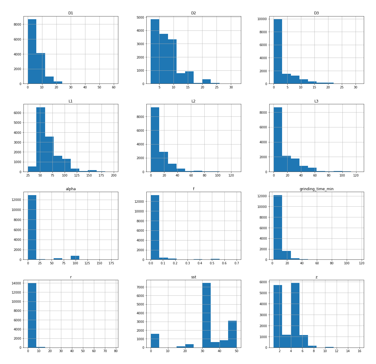
Figure 2: Feature distribution histogram
Next, we had a look at which parameters influenced the grinding time significantly and which parameters could safely be ignored. One very simple way to do so visually is to plot a correlation matrix of all our parameters. This creates a matrix of all parameters; each cell tells us how closely they correlate over the data set. 1 means they move in sync, 0 that they don’t correlate at all. We’re particularly interested in the grinding_time column: It tells us which parameters have the most influence on it. Contrary to what we assumed, the materials didn’t have a significant impact, so we removed them from the training data, making the training and tuning process faster. Figure 3 shows a correlation matrix with the materials already dropped. We can see that D2, D1, L2 and L1 are the most significant factors.
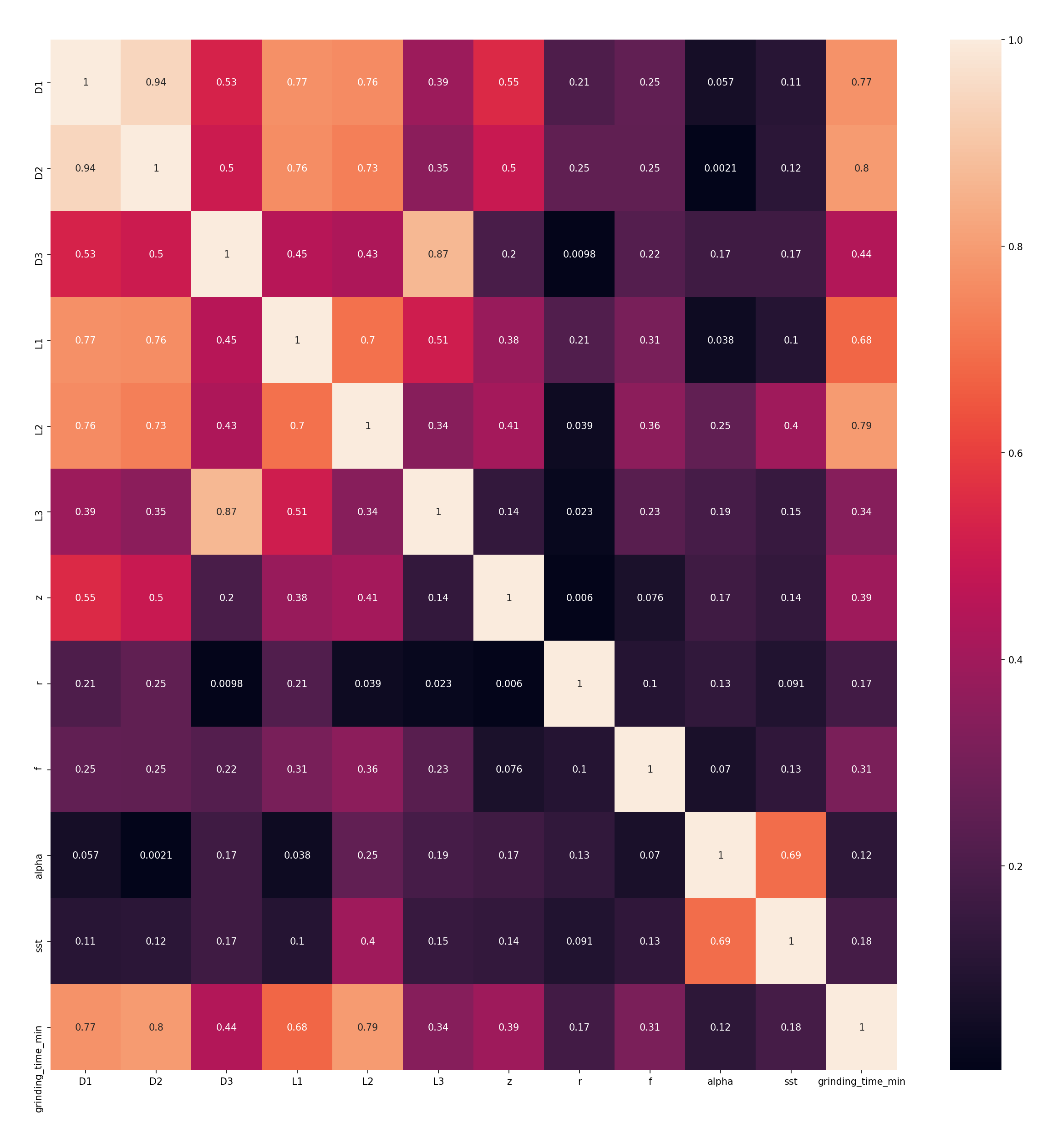
Figure 3: Feature correlation matrix
You can’t overestimate the value these data-aided discussions with people who understood the domain brought to the table. Without them, we wouldn’t have been able to tell apart edge cases from actually faulty data. With the right people looking at the data, it was simple. While combing through the raw data set is not something you can ask your experts to do, identifying irregularities and then looking at specific data points yields a more thorough understanding quickly.
To plot the figures, we used matplotlib[4] seaborn[5]. Listing 2 and 3 show how trivial it is to generate visualizations from a pandas dataframe.
Confident our training data made sense, we set out to train some models and see whether we could get accurate results.
Model training
Dividing our data set into label label (the feature we’re looking for, i.e. the grinding time) and remaining features and training/validation data is easily accomplished using tools from the scikit-learn[6] library. We settled for a simple 80%/20% train/test split.
To find out a suitable model, we compared three different ones: Linear Regression, to get a simple baseline, Random Forest Regression[7], and XGBoost[8]. Out of these three, linear regression performed worst at 80% accuracy. Without tweaking, the other two scored an accuracy of between 85% and 90% with a mean error of roughly 2.5 minutes. Not bad as a starting point. Not bad at all.
To increase the accuracy, we tuned the respective model’s hyperparameters experimentally using hyperopt[9], a python library for parameter optimization.
Picking the best hyperparameter combination from the optimization runs and re-training the two remaining models with them allowed us to increase their accuracy to 91.25% (random forest) and 91.45% (xgb), respectively.
All of these libraries can be used with scikit-learn seamlessly making model selection and evaluation very approachable, even for developers with limited machine learning experience.
It is important to note that looking over the data with domain experts to purge implausible data points yielded an increase in model accuracy of ~10%, while hyperparameter optimization only yielded 1-5%. Even with clever statistic tools at hand, it’s important to have people actually understanding the business in the loop. Who would have thought…
To make sure the model’s predictions match the expectations, we used the trained model to predict all grinding times of the complete data set, compared it with the actual recorded times, and discussed the data points with the highest deviation again. This allowed us to identify additional needs for simulation data and implausible data points we missed earlier. The following figures show the results for both models. If the model were 100% accurate, all points would fall together with the grey line. We also exported the results into Excel to allow our domain experts to easily look at all the parameters for a prediction to judge whether unexpected results could be explained.Both models have similar accuracy, but we can see that the error profile of the XGBoost model looks better. This is why we picked that one to include in our price calculation algorithm. There are still some predictions that are significantly off, but that’s not a problem: Since the grinding time is but one factor in the overall price calculation, outliers can be identified and cut off at certain points.
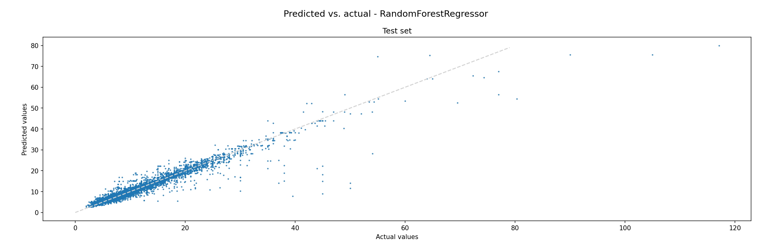
Figure 4: Random Forest predicted vs. actual values
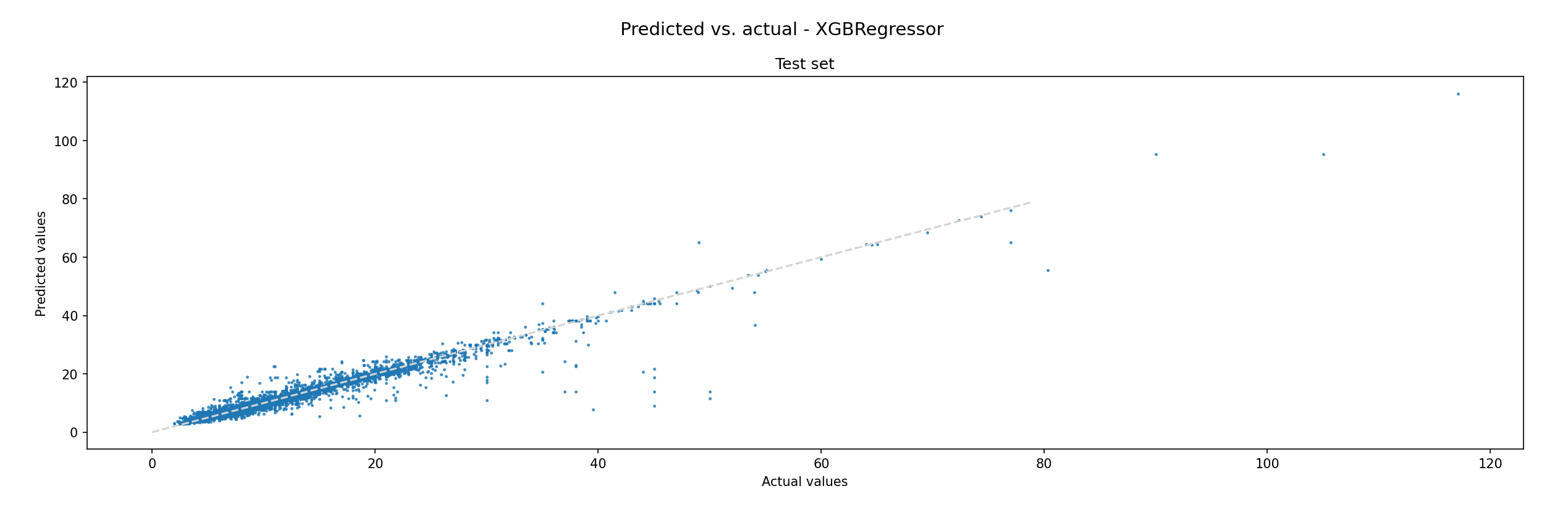
Figure 5: XGB predicted vs. actual values
Applying the trained model
With that, we had a fully trained and evaluated model at our hands, the only thing left to do was to integrate it into our applications. m2cgen [10] is a library to generate code in a plethora of languages from trained statistical models. Listing 4 shows how to generate Java code from a model and write it to a file. We built a thin wrapper around the generated code so it would accept the parameters in the format returned from the online configurator and exposed it via an HTTP API.
Success factors & conclusion
It is interesting to note is that this project didn’t start out as a machine-learning initiative. We were facing a challenge and had enough sample data at our hands. Given that, machine learning simply was the most promising approach.
You might be tempted to think this endeavor required highly specialized staff, but none of the developers involved with the project had prior production experience with machine learning. Data science and machine learning documentation and tooling have become much more approachable during the last few years, so we could simply take off-the-shelf open-source libraries and pick up the required know-how as we went along.
Including domain experts in the data preparation process from the beginning was crucial. As noted earlier, the biggest improvement of the model was due to identifying which data points were accurate and which ones needed to be discarded.
If we hadn’t modeled our work logging solution as an event-sourced system, the data required would not have been available to us. Gathering that data by experiment or simulations alone would have been either prohibitively expensive and/or wouldn’t have given us a data set having the required size and quality.
As the event log grows, so does the size of the training data set. By repeating the training process outlined above with an updated training set will allow to further increase the model’s accuracy. Additionally, reviewing predictions, comparing them with actual grinding times, and feeding the result back into the training process can be used as an additional enhancement, if need be. This could even be done in an automated fashion using continuous integration (CI) pipelines, making the model more accurate without human interaction.
The described case is tailored to custom tool manufacturing, however, the general approach can be utilized in similar scenarios as well. We’re looking forward to digging deeper into our event streams to gain more insights into our production processes in the future.
Listings
Listing 1: Grinding time projection
fromStream('worklogging')
  .when({
    $init: function () {
      return {}
    },

    ['grinding-stopped']: function (s, e) {
      if (!e.data.durationSeconds) return s// ignore events with missing grinding times
      if(! (
        e.data.context
        && e.data.context.order
        && e.data.context.order.artNo
      )) return s // skip trackings w/o article number

      s[e.metadata.source_event_id] = {
        grindingTime: e.data.durationSeconds,
        artNo: e.data.context.order.artNo
      }
	  return s
    },

    ['event-reverted']: function (s, e) {
      if (e.data.revertedEventProperties === 'grinding-stopped') {
      delete s[e.metadata.source_event_id]
	  return s
    }
  },
})
.transformBy(function (state) {
  return Object.values(state)
})
.outputState()
Listing 2: Histogram
# df is the pandas data frame containg our sample data
cols = ['D1','D2','D3','L1','L2','L3','z','r','f','alpha','sst','grinding_time_min'] # specify columns to plot
df[cols].hist(figsize=(20,20));
Listing 3: Correlation matrix
import seaborn as sn
import matplotlib.pyplot as plt

fig, (ax) = plt.subplots(1, 1, figsize=(20, 20), dpi=150) # scale the image to a reasonable size

sn.heatmap(df[cols].corr().abs(), annot=True)
Listing 4: Generate Java code
code = m2c.export_to_java(model, indent=2, function_name="predictGrindingTime")

with open('./Model.java','w') as f:
    f.write(code)
    f.close()